DC-Machine Experiment
-
Introduction
-
Theory
-
Controller
-
Windup effect & Anti Windup
-
Preparation
-
Videos
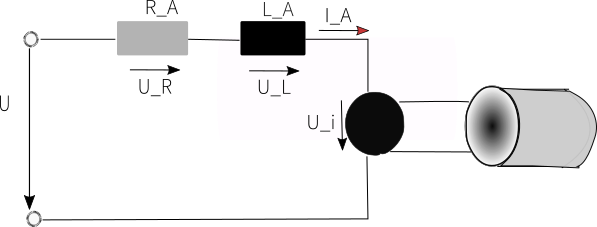
The DC motor, also called continuous current motor, belongs to the class of electric motors and is mainly used to convert electrical energy into mechanical energy. Most forms of DC motors are based on magnetic forces in this context and have internal mechanisms of an electronic or electromechanical type. A continuous current electric machine is made up of:
- a stator which is at the origin of the circulation of a fixed longitudinal magnetic flux created either by stator windings or by permanent magnets. It is also called an “inductor” in reference to the generator operation of this machine.
- a wound rotor connected to a rotating commutator reversing the polarity of each rotor winding at least once per revolution so as to circulate a transverse magnetic flux in quadrature with the stator flux. Rotor windings are also called armature windings, or commonly “armature” in reference to the generator operation of this machine.
1. How does a DC-Machine work?
The working principle of the DC motor is as follows: An electric current flows through a coil in a magnetic field, then the magnetic force generates a torque that makes the DC motor turn.

2. Control of a DC-Machine
Controllers automatically influence the physical variables in a mostly technical process in such a way that a specified value is maintained as well as possible even in the presence of disturbances.

A closed-loop control System is a technical device designed to automatically Keep a controlled variable Y (Output) at a defined value, the reference variable w (Input). The aim of the closed-loop control system is to use an Actuator to minimise the control deviation e even under the influence of disturbance variables.
Why do we need a Control loop?
The control loop describes the self-contained process for influencing the controlled variable x so that the controlled variable x reaches and maintains the value of the reference variable w. In the control loop we speak of a continuous sequence of measuring – comparing – adjusting.
3. The transfer function
How does a simple transfer function of a DC-Machine in its linear operating range works?
Determining Input/ Output
Input: Voltage U(t)
Output: Speed W(t)
Modelling of electrical part
U(t)= U_R(t)+U_L(t)+U_i(t) ;
L_A \cdot \frac{dI_A(t)}{dt}+ U_R(t)+ U_i(t) ;
U_i(t)= C_e \cdot W(t) ;
M(t)= C_m \cdot I(t) ;
W(t)= \frac{1}{J_{system}} ∫ M dtModeling of mechanical part
J_{system} = J+ m\cdot r² with J, Ring disc
Laplace Transformation: Determination of the induced current
U(S) – I\cdot R – S \cdot L\cdot I – U_i(S)= 0 ;
U(S) – U_i(S) = I(R+S\cdot L) ;
I(S)= \frac{U(S) – U_i(S) }{R + S\cdot L}Step response
H(S) = \frac{I}{U(S) – U_i(S) } = \frac{1}{R + S\cdot L }Determination of the Speed
W(S) = M(S)\cdot \frac{1}{J_{system}\cdot S}1. Type of Controller
Proportional gain
The P-controller consists exclusively of a proportional part of the gain K_p. With its output signal it is proportional to the input signal. Because of the lack of time response, the P-controller responds immediately, but its use is very limited because the gain must be greatly reduced depending on the behavior of the controlled system.
Integral gain
An I-controller (integrating controller, I-element) acts by time integration of the control deviation e(t) on the manipulated variable with the weighting by the reset time. Due to its (theoretically) infinite gain, the I-controller is an accurate but slow controller. It leaves no permanent control deviation. Because it inserts an additional pole in the transfer function of the open loop and causes a phase angle of -90° according to the bottom diagram, only a weak gain K_s or a large time constant T_n can be set.
2. Dimensioning the controller (Chien, Hrones, Reswick)
The adjustment rules according to Chien, Hrones and Reswick are an approach developed in 1952 for the favorable adjustment of controllers. They are considered a further development of the second method of Ziegler and Nichols. Advantageously, the control parameters are separated for favorable disturbance and guidance behavior. They are likewise subdivided for aperiodic or periodic controls.
PI-Regler: R(S) = \frac{Kr}{1 + \frac{1}{T_n\cdot s}}

How to determine T_u (delay time), T_g (compensation time) and K_s (stationary gain)?
It can be done in 3 steps:
- First is creating step response.
- Second is creating the first derivative of step response.
- Third is creating the tangents of step response at the point where the value of the first derivative is largest.
The final value of the step response is K_s . The abscissa of the intersection of the tangent and the x-axis is T_u . The abscissa of the intersection of tangent and step response – Tu is T_g

Windup-effect
Compared to ideal systems, real systems have some undesirable effects, such as nonlinearity, the feedback variable with measurement uncertainty, and more often some of them are saturated. So if the manipulated variable of a control loop is saturated and the controller has the I component, then as a side effect, the I component integrates away. The consequence is that the process cannot be controlled for a longer period of time (Wundup).
Anti-Windup
The anti-windup circuit offers a possibility to prevent this. The aim is to stop or at least weaken the integration process as soon as the manipulated variable is in saturation. One method of overcoming the winup effect that you could use in this test is to limit the I component to the level of the available control signal.
Graphic representation of Windup & Anti-Windup
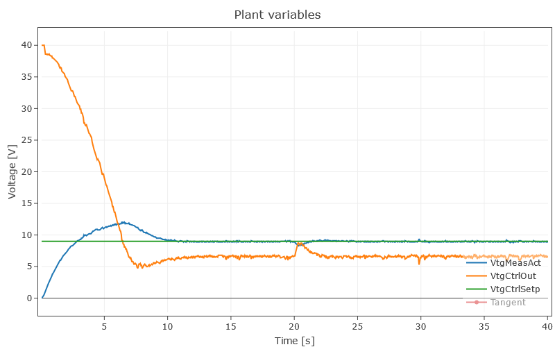
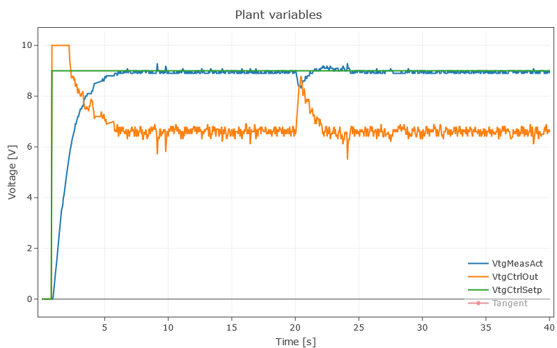
Figure 5 shows that the manipulated variable integrates away up to about 40 V due to the I-component. Thereby the actual value stabilizes after a long time interval in comparison to figure 6, where it comes to rest after a very short time (here approx. 6 s).
About the experiment
This graph shows an overview of the control loop, which we will study in this Versuch. let it work on you before you start experimenting
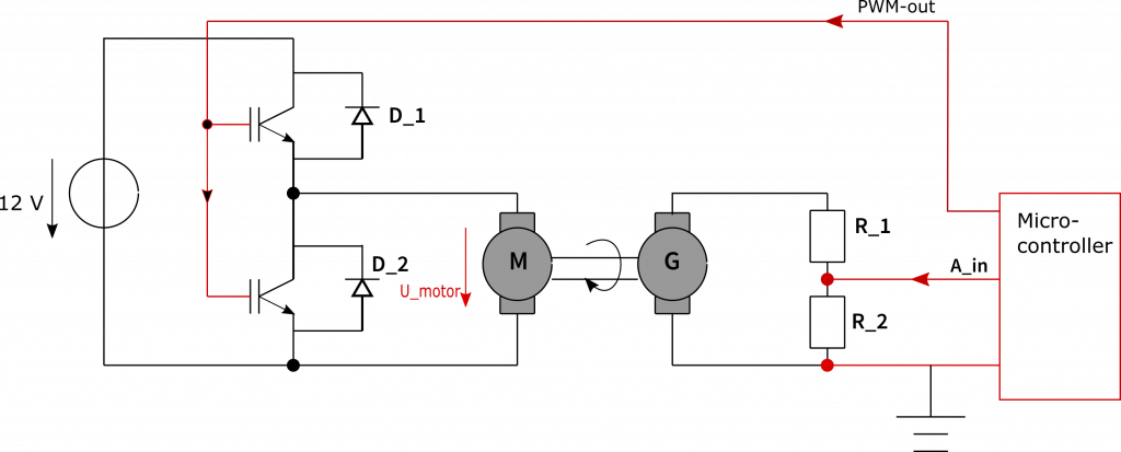
G= Genator, M= Motor
In this test it will be a question of calibrating the controller for the control of the speed of a DC motor with the method of inversion of the tangent and definition of the rules according to Chien, Hrones and Reswick.
Step 1. Recording the step response
Determine the transfer behavior of the line by recording a step response and determining the parameters K_s, T_g and T_u from it (sees rider controller).
Step 2. Determine controller parameters
Determine the parameters of the PI-controller, as well as the optimized guide parameters. The table of parameters can be found in the Controller tab.
Step 3. Model a control loop with PI-controller and anti-windup unit.
Now model a control loop with a PI-controller and with an anti-windup device using the parameterized process model. You should design the controller yourself and anti-windup should be deactivatable.
The motor voltage is limited to ±12 V , please provide for this in your controller.
There are various anti-windup methods – limiting the I component to a fixed portion of the possible actuating signal is probably the simplest option – but there are no limits to your creativity here