Experiment #2: Floating ball (test)
Introduction
Floating ball is a system in which a ball is controlled at a certain height in a plastic tube with the help of a DC motor with a 30 mm propeller and a suitable controller.
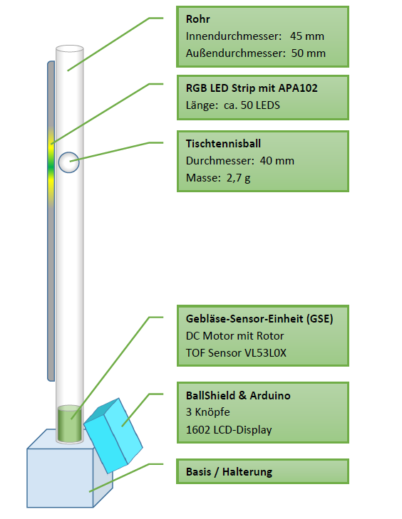
The floating ball system includes the following elements: a Laser based sensor, the Arduino Mega 2560 microcontroller, a DC-20-8.5 motor with a 30 mm propeller, an LCD with I2C expander, an RGB LED strip with APA102 and a BallShield for Arduino Mega.
With the question how does the floating ball work, we will create a detailed overview in this topic. Secondly, it will be shown how to determine the transfer function and the control of the floating ball. After that, we will talk about the dimensioning and implementing of the controller. Finally, with all this knowledge you will be able to perform the experiment in the last tab right.
Theory
1. How the floating ball work?
In this floating ball experiment, a ping-pong ball is controlled at a certain height in a Plexiglas tube. The tube is about 800 mm high, and the ball is propelled to a certain height by an air flow using a motor with a propeller. In the lower part of the tube are the power electronics (for example on the Ball Shield) and the microcontroller (figure …).
2. Control of a floating ball
Controllers automatically influence the physical variables in a mostly technical process in such a way that a specified value is maintained as well as possible even in the presence of disturbances.

A closed-loop control System is a technical device designed to automatically Keep a controlled variable Y (Output) (here the set value of the height of the ball ) at a defined value, the reference variable w (Input) (the actual value of the height of the ball). The aim of the closed-loop control system is to use an Actuator to minimise the control deviation e even under the influence of disturbance variables.
3. Why do we need a Control loop?
The control loop describes the self-contained process for influencing the controlled variable x so that the controlled variable x reaches and maintains the value of the reference variable w. In the control loop we speak of a continuous sequence of measuring – comparing – adjusting.
The transfer function of floating ball
Let us consider the system shown above (Figure…) in the static area, i.e. the ball is at a certain height and remains constant there. Then, from a physical point of view, we can use Newton’s first law to describe the system, which says: \sum\vec{F} = \vec{0} . We can analyse the forces acting on the system of a floating ball:
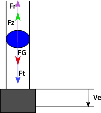
In figure 3, 4 different forces act on the ball:
- he weight force: F_{G}= m\cdot g
- The mass inertia force: F_{t}= m \cdot \dot{z}
- The friction force F_{r}= 6 \cdot \pi \cdot r \cdot \mu_{0}\cdot v
- The tractive force: F_{z}= \delta p \cdot A_{b}
where:
m : mass of the ball
g : acceleration due to gravity
\ddot z : the second time derivative of the
altitude
r : the radius of the ball
\mu_{0} : the dynamic viscosity of air
v : the resulting velocity
means( vl − \dot z ) velocity of the air
minus velocity of the ball.
\delta p : the difference in air pressure between the
upper and lower part of the ball
A_{p} : the cross-sectional area of the ball
thus results in : F_{z} + F_{r} – F_{g} -F_{t} =0 (1)
How does a simple transfer function of a floating ball in its linear operating range works?
- Determining Input/ Output
Input: Voltage V_{e}(t)
Output: the vertical position of the object in the tube z(t)
- Transfer function
The next step is to replace each parameter in equation (1) with its value
By using equation (1), the transfer function can be easily found.So to deduce it, we must proceed as follows:
- First of all, put equation (1) in the form of a differential equation
- we learned in control enginnering that to easily solve the differential equation (in the time range) obtained it will be necessary to transform it into a Laplace transform (Laplace Transformation: U (t) gives U(S) with Laplace in the frequency range)
- After having obtained the Laplace transform of the equation, the output value is derived from the input value, ( H(S)= \frac{Z(S)}{V(S)} ) and this corresponds to the transfer function H (S)
Notes: the differential equation found from equation (1) must be linearized, because it is a 2nd order differential equation
Controller
1. Type of Controller
- P-Controller:
The P-controller consists exclusively of a proportional part of the gain Kp. With its output signal it is proportional to the input signal. Because of the lack of time response, the P-controller responds immediately, but its use is very limited because the gain must be greatly reduced depending on the behavior of the controlled system.
- I-Controller:
An I-controller (integrating controller, I-element) acts by time integration of the control deviation e(t) on the manipulated variable with the weighting by the reset time. Due to its (theoretically) infinite gain, the I-controller is an accurate but slow controller. It leaves no permanent control deviation. Because it inserts an additional pole in the transfer function of the open loop and causes a phase angle of -90°−90° according to the bottom diagram, only a weak gain Ks or a large time constant can be set Tn.
- D-Controller
The D controller evaluates the change of a control deviation (it differentiates) and thus calculates its rate of variation.
Because of the different advantages of the PID controller, it is used in this experiment to control the ball to a setpoint.
2. Dimensioning the controller
The controlled system in the Schwebe ball experiment is a PT1 element so the appropriate controller used here to hold the ball at a certain height is the PID controller. For the dimensioning of this Regler, we will use the method of Ziegler Nichols Stabilitätsrande.
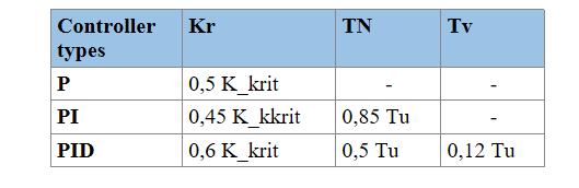
The formula of the PID controller is as follows:
R(S)= K_{r} (1+ \frac{1}{T_{n}\cdot S}+ T_{v}\cdot S ) (2)
When dimensioning the controllers according to Ziegler, the following is done:
- First determine the factor Kkrit
- Then, with the help of this factor and the table below, determine the Kr, Tn and Tv (see table 1 below)
- Then the values are used in the equation (2) to determine the values of the controller
How to determine K_krit
The controller is closed by means of a P-controller
The controller gain is increased until the closed circuit performs continuous oscillations. The resulting gain is referred to as Kkrit (See figure below).
Preparation
About experiment
This graph shows an overview of the control loop, which we will study in this Versuch. let it work on you before you start experimenting
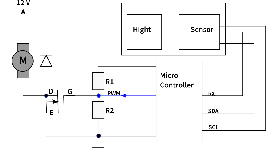
This test is about setting the controller to control the speed of a ball using the Ziegler-Nichols method of stability rand. to do this, the following procedure must be followed:
- oscillation method according to Ziegler-Nichols
Use P-controller to find the critical gain
K_{krit} and the associated period t_{Tu} at a setpoint of 12 V (with Matlab).
Note: t_{Tu} is the duration of a period on the graph that you got
Krit ermittelt, periode von schwingung, Pid auslegen
2. controller configuration/ setting rules from Ziegler Nichols
Use the table above (Controller types) to determine the parameters of the PID controller
Then put this parameter into equation 2 to determine the value of the PID controller.
Then with these values launch experiment and see how the ball behaves